Conditional formatting helps users analyze data and visualize it. Radio buttons in Excel allow you to add a simple formula depending on the requirements.
Benefits of using Radio button conditional formatting.
- Users can easily switch views with different perspectives.
- Its user-friendly usage.
- Use it for different data types.
Step-by-step guide to use it with example.

Step 1: Create a new file and enter data as shown in the image. Click on the developer tab, insert option, then radio button. Change the title according to you.

Step 2: Right-click on Radio button, click on format control, check the box, and link all radio buttons to the same cell as in image.

Step 3: Select the data, click on conditional formatting – new rule- format style (data-bar)- type as formula in both minimum and maximum. Add the formula as shown in the image, where (02) is the cell number where we have linked all radio buttons. Add color of your choice.

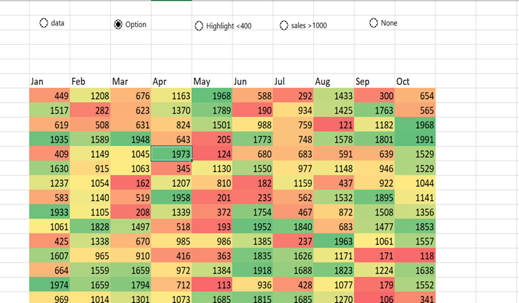
Step 4. Click on the second radio button, click on conditional formatting – new rule- format style (3 color scale)- type as, and use the formula as shown in the image above. (3,4,5).
Step 5: Click on the 3rd radio button – click on conditional formatting – select rule type as shown in image.

Step 6: Click on the 4th radio button – click on conditional formatting – select rule type as shown in the image.

Note: We have added conditions like highlight< 400 and sales> 1000 in radio buttons 3rd and 4th, respectively. You can try with different conditions. C7 is starting for the numbers I have added
Hemant is Digital Marketer and he has 6 + years of experience in SEO, Content marketing, Infographic etc.